function [yhat,omega]=ft_approx(y,a,b)
% FT_APPROX computes an approximate Fourier transform from samples
% contained in the vector y. The arguments a and b are the intial
% and final times for samples to be taken. The outputs are the
% approximate Fourier transform, contained in yhat, and the
% corresponding frequencies, contained in omega. The frequencies
% are in radians per second.
%
% F. J. Narcowich, Mar. 20, 2012.
%
s=size(y);
y=y(:).';
N=floor(length(y)/2);
if N < length(y)/2,
    M=N;
else
    M=N-1;
end
dt=(b-a)/(2*N);
del_omega=2*pi/(b-a);
omega=((-N):(M))*del_omega;
phase_factor=exp(-i*a*omega);
yhat=phase_factor.*fftshift(fft(y))*(dt/sqrt(2*pi));
yhat=reshape(yhat,s);
omega=reshape(omega,s);
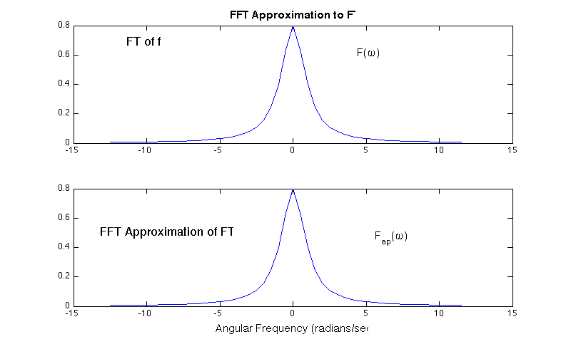
Solution First define f and its Fourier transform in matlab
using the ``anonymous'' function method:
f = @(x) exp(-abs(x))
fhat = @(x) sqrt(2/pi)*(1+x.^2).^(-1)
Next, define arrays for dealing with n = 2L time
samples.
n=2048;
t=(-2*pi):4*pi/n:(2*pi - 4*pi/n);
y=f(t);
Finally, find the approximate FT, yhat, and the values of the
frequency on which it is calculated, omega. Do the same for the actual
FT, and then plot the results. (The variable ind
restricts the points plotted to a small frequency band about ω =0.)
[yhat,omega]=ft_approx(y,-2*pi,2*pi);
yhat_actual = fhat(omega);
ind=1000:1048;
subplot(2,1,1), plot(omega(ind),yhat_actual(ind))
subplot(2,1,2), plot(omega(ind),real(yhat(ind)))
Updated 3/21/2014